PathEffects: Enhancing Matplotlib Artists

In Matplotlib, PathEffects are powerful tools that allow you to modify how artists (like lines, patches, and text) are drawn at a low level. They affect the artist’s path properties during the rendering process, enabling effects such as outlines, shadows, or modified strokes.

The mpl_visual_context.patheffects module significantly extends Matplotlib’s native PathEffects system. It provides a rich collection of additional, often composable, effects designed to make sophisticated visual customizations more accessible. Whether you want to add a subtle highlight, create a striking glow, or apply complex layered effects, this module provides the building blocks.

This guide will walk you through the various PathEffects available in mpl-visual-context, demonstrating how to use and combine them to achieve unique visual outcomes in your Matplotlib plots.

Composable PathEffects

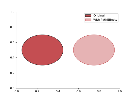
One of the core strengths of mpl_visual_context.patheffects is the concept of composable PathEffects. Many effects inherit from ChainablePathEffect, allowing them to be pipelined using the | (pipe) operator. This enables you to build sophisticated custom effects by combining simpler ones in a clear and readable way. For example, you could first modify an object’s color, then apply a stroke-only effect.

import matplotlib.pyplot as plt
from mpl_visual_context.patheffects import (HLSModify,
                                            StrokeColorFromFillColor,
                                            FillOnly, StrokeOnly)

fig, ax = plt.subplots()

# original
p1 = plt.Circle((0.25, 0.5), 0.2, fc="r", ec="k", label="Original")
ax.add_patch(p1)

# w/ patheffects
p2 = plt.Circle((0.75, 0.5), 0.2, fc="r", ec="k", label="With PathEffects")
ax.add_patch(p2)

# 1. Modify lightness and then render with fill only (no stroke)
pe_fill = HLSModify(l=0.8) | FillOnly()
# 2. Use the original fill color for the stroke, then render with stroke only (no fill)
pe_stroke = StrokeColorFromFillColor() | StrokeOnly()

p2.set_path_effects([pe_fill, pe_stroke])
ax.legend()
plt.show()

(Source code, png, hires.png, pdf)

Below is a categorized list of available chainable PathEffects.

Color-Related Effects

These effects modify the colors (fill or stroke) of an artist.

HLSModify	PathEffect which modifies the color in HLS space.
HLSaxb	PathEffect which modifies the color in HLS space.
ColorMatrix	PathEffect which modifies the color in RGB space, using a predefined color matrix.
FillColor	PathEffect to set the fill color
FillColorFromStrokeColor	PathEffect to set the fill color by the stroke color
StrokeColor	PathEffect to set the stoke color
StrokeColorFromFillColor	PathEffect to set the stoke color by the fill color

Path-Related Effects

These effects alter the geometry or rendering style of the artist’s path.

StrokeOnly	PathEffect with only stroke.
FillOnly	PathEffect with only fill.
Open	PathEffect with no closed with.
Partial	PathEffect with that preserve only a part of the path.
Smooth	PathEffect that transform the given lines to smooth bezier path.
SmoothFillBetween	PathEffect that transform a patch created by fill_between to a smooth nezier path.

Clip-Related Effects

These effects deal with clipping an artist’s path.

ClipPathFromPatch	PathEffect that clips the path using a provided patch.
ClipPathSelf	PathEffect that sets the clip_path to the path itself.
ClipRect	PathEffect that modifies the clip_rect using the given coordinate (and transform).

Transform-Related Effects

These effects apply transformations to the artist’s path.

Offset

PathEffect that offsets the path.

Multiple Strokes & Glow Effects

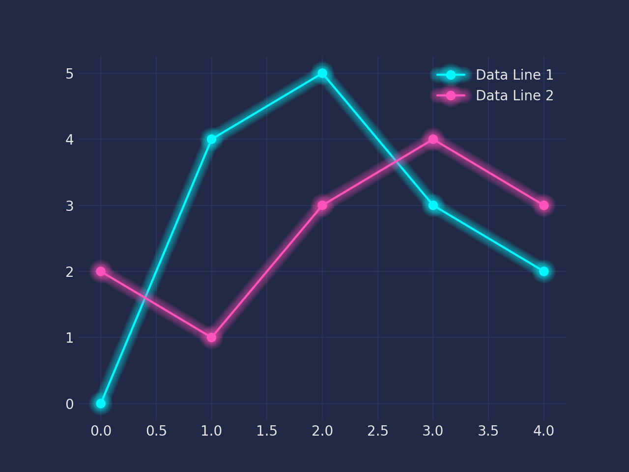
Achieve striking visual styles like glows or multiple outlines, often inspired by cyberpunk aesthetics or used for emphasis. These effects typically involve drawing the artist’s path multiple times with varying styles.

import matplotlib.pyplot as plt
import mplcyberpunk
plt.style.use("cyberpunk") # Using cyberpunk style for thematic background/colors
from matplotlib.patheffects import Normal
from mpl_visual_context.patheffects import Glow

fig, ax = plt.subplots()

l1, = ax.plot([0, 4, 5, 3, 2], "o-", label="Data Line 1")
l2, = ax.plot([2, 1, 3, 4, 3], "o-", label="Data Line 2")

# Apply Glow (draws multiple faint lines) then Normal (draws the original line on top)
glow_effect = [Glow(n_glow_lines=10, alpha_line=0.6), Normal()]
for l in [l1, l2]:
    l.set_path_effects(glow_effect)
ax.legend()
plt.show()

(Source code, png, hires.png, pdf)

Available effects for multiple strokes:

Glow	Patheffect with glow effect.
CmapGlow	Patheffect similar to Glow, but with different colors basedon the given colormap.

Image-Based PathEffects (e.g., Gradients)

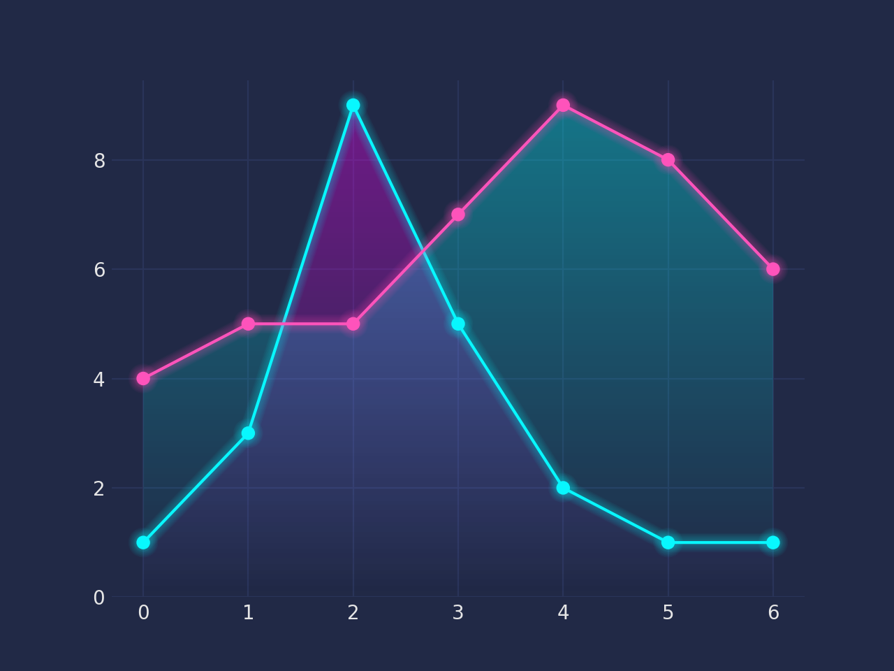
Some PathEffects in this library don’t just alter paths; they draw images. A notable application is creating gradient effects. These effects often leverage an underlying “ImageBox” concept for generating the necessary image data.

For instance, AlphaGradient can be used to create a fill that fades out, which is useful for highlighting regions or creating depth.

Note

The term “ImageBox” refers to an internal mechanism or a closely related set of tools within mpl-visual-context responsible for generating image data (like gradients) that these PathEffects can then use. While not always a separate, user-facing module, understanding this concept helps clarify how these effects work.

import matplotlib.pyplot as plt
import mplcyberpunk
plt.style.use("cyberpunk") # Using cyberpunk style for thematic background/colors
from matplotlib.patheffects import Normal
from mpl_visual_context.patheffects import Glow, AlphaGradient

fig, ax = plt.subplots()
x = range(7)
y1 = [1, 3, 9, 5, 2, 1, 1]
y2 = [4, 5, 5, 7, 9, 8, 6]

l1, = ax.plot(x, y1, marker='o')
l2, = ax.plot(x, y2, marker='o')
p1 = ax.fill_between(x, y1, alpha=0.6, color="magenta") # Base fill for context
p2 = ax.fill_between(x, y2, alpha=0.6, color="cyan")    # Base fill for context

# Apply Glow to lines
line_glow = [Glow(n_glow_lines=8), Normal()]
for l in [l1, l2]:
    l.set_path_effects(line_glow)

# Apply an upward AlphaGradient to the filled areas
# This will make the fill_between areas fade upwards
fill_gradient = [AlphaGradient("up")]
for p_fill in [p1, p2]: # Renamed p to p_fill to avoid conflict
    p_fill.set_path_effects(fill_gradient)
ax.set_ylim(bottom=0) # Ensure gradient direction is clear
plt.show()

(Source code, png, hires.png, pdf)

Available image-based PathEffects:

AlphaGradient	Fill the path with image of the fill color of the path, with varying transparency.
Gradient
FillImage	Fill the path with the given image.

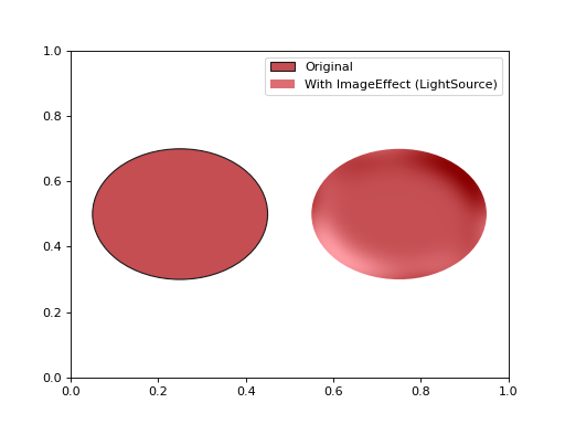
ImageEffect: Applying Image Filters

The ImageEffect is a special PathEffect that brings raster image processing into the Matplotlib rendering pipeline. It works by first rendering the artist (along with any preceding PathEffects in a chain) into an image buffer using Matplotlib’s Agg backend. Then, an image processing filter (e.g., Gaussian blur, lighting effects) is applied to this buffer. Finally, the modified image is drawn onto the canvas.

This is particularly useful for effects that are difficult or impossible to achieve with vector graphics alone, such as realistic blurs or complex lighting.

Important: ImageEffect can be pipelined but should generally be placed at or near the end of a PathEffect chain. It can even follow non-chainable PathEffects.

import matplotlib.pyplot as plt
from mpl_visual_context.patheffects import FillOnly, ImageEffect
from mpl_visual_context.image_effect import LightSource # Example image filter

fig, ax = plt.subplots()

# Original for comparison
p1 = plt.Circle((0.25, 0.5), 0.2, fc="r", ec="k", label="Original")
ax.add_patch(p1)

# With ImageEffect
p2 = plt.Circle((0.75, 0.5), 0.2, fc="r", ec="k", label="With ImageEffect (LightSource)")
ax.add_patch(p2)

# Apply FillOnly, then ImageEffect with a LightSource filter
light_effect = FillOnly() | ImageEffect(LightSource(erosion_size=5, gaussian_size=10))
p2.set_path_effects([light_effect])
ax.legend()
plt.show()

(Source code, png, hires.png, pdf)

Available ImageEffect:

ImageEffect